How You Can Convert Rows to Columns or Columns to Rows in Excel Worksheet

Updated on: September 03, 2022 | Teachable Tech

In Microsoft Excel, you can easily convert rows to columns or columns to rows in Excel Workbooks, and either uses the Transpose or Transpose function to get the output. The transpose function normally returns a transposed range of cells, which is used to switch the rows to columns and vice versa. I.e., we can convert vertical cells to a horizontal range of cells or horizontal cells to a vertical range of cells in Excel.

There are two different methods for converting rows to columns in Excel, such as:

Transposing Columns to Rows Using Paste Special.
Transposing Columns to Rows Using TRANSPOSE Formula.

Using Paste Special

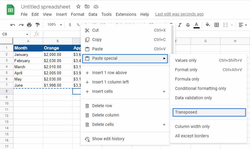
Here, we have some records of sales for some of the products (apple, orange, and cherry) for the months from January to June. We will try to convert the columns into rows so that we can visualize the records for the months as column headers, and we will utilize this dataset mainly to demonstrate the ways of converting multiple rows to columns easily.

The following steps convert rows to columns in Excel using the Paste Special method:

Select the whole dataset that needs to be transformed or transposed. Then, copy the selected data by simply pressing the Ctrl + C keys.
Then click on a blank cell where you want to copy the transposed data, and the cell you select becomes the top-left corner of whatever you are copying.
Then click on a blank cell where you want to copy the transposed data, and the cell you select becomes the top-left corner of whatever you are copying.
Now, Click the down arrow under the Paste option, and then click the Transpose button on the drop-down menu.
Then, you will be able to transpose your data, which means converting the columns into rows.

Using TRANSPOSE Formula

In this section, we will use a TRANSPOSE array function to convert the following dataset's multiple rows into multiple columns and then gather the data. This array function works the same way as transpose. I.e., we can convert rows to columns and vice versa and also format another table below the main dataset.

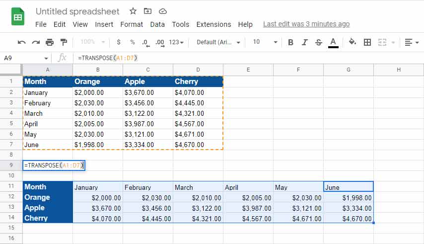
The following steps convert rows to columns in Excel using TRANSPOSE formula:

First, count the number of columns and rows in your original excel table and then select the same number of blank cells, but ensure you have to transpose the columns to rows like in above Examples. Choose the blank cells in the opposite direction and the number of rows is 3, and the number of columns is 6. So, you will select 3 blank columns and 6 blank rows.
In the first empty cell, enter the TRANSPOSE formula in excel ‘=TRANSPOSE(A1:D7)’.
This formula needs to be applied to other blank cells, so press ‘Ctrl+Shift+Enter.’
After completing all the steps, the rows are converted to columns.

The Paste Special method is useful when the user needs the original formatting to be continued and, by using the TRANSPOSE function, the converted table will change its data automatically, which means that whenever the user changes the data in the original table. It will automatically change the data in the transposed table as it is linked.